
|
Preparing for the SAT? Claim Your Personalized Math Plan →
|
In mathematics and statistics, linear regression is a method for modeling the relationship between two variables using a straight line — called the line of best fit — that best represents the trend in a scatter plot. The regression equation is written as ŷ = a + bx, where b is the slope (rate of change) and a is the y-intercept (predicted value when x = 0). Linear regression appears in Florida’s MAFS.912.S-ID.6 standards, AP Statistics, and the SAT Math Problem Solving & Data Analysis section.
Linear regression models the relationship between two variables with a straight line, the line of best fit, that best represents the trend in a scatter plot. The equation is ŷ = a + bx, where b is the slope (rate of change) and a is the y-intercept (predicted value when x = 0). Tested on the SAT Math “Problem Solving & Data Analysis” section.
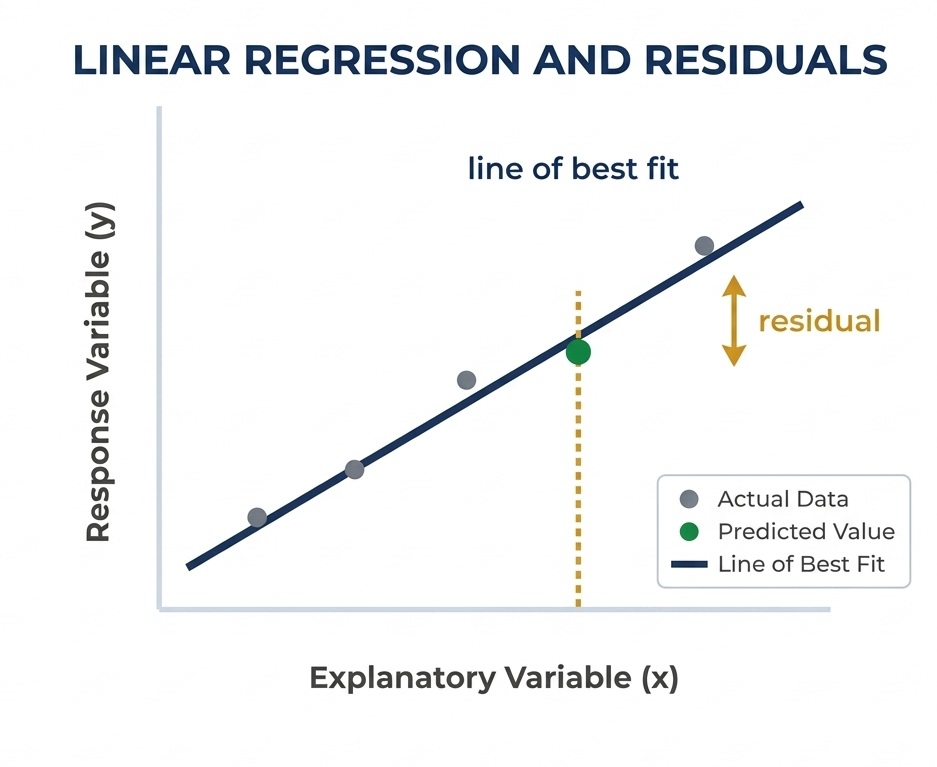
Linear regression is a statistical method for finding the straight line that best models the relationship between two quantitative variables. This line , the regression line or line of best fit , minimizes the total distance between itself and all the data points. The equation predicts the dependent variable (ŷ, “y-hat”) for any value of the independent variable x, making it a tool for both analysis and prediction.
Calculator tip: on the SAT calculator section, plug the data points into a DESMOS table and use its regression feature to get the equation instantly: faster and less error-prone than a TI-84[cite: 8].
Same structure as slope-intercept form, different notation. Interpreting what each part means in context is the skill the SAT actually tests,not memorizing the equation.
Interpret the slope in context: "for every 1-unit increase in x, ŷ increases/decreases by b": always in real-world units. For ŷ = 12.5 + 3.2x (x = study hours, ŷ = test score): each extra hour adds a predicted 3.2 points. The SAT's "what does 3.2 represent?" answer is always a rate[cite: 9].
TI-84 vs. statistical notation: the TI-84's LinReg output shows "y = ax + b" where a = slope, b = intercept: the opposite of AP Statistics notation (ŷ = a + bx, where a = intercept)[cite: 9]. Don't copy blindly. Identify slope by position: the coefficient of x is always the slope, whatever letter the calculator uses[cite: 9].
SAT insight: a negative y-intercept isn't an error — 0°F is just outside the data range, so the intercept has no real-world meaning here. Focus on what the slope represents.
Remember: Residual = Actual − Predicted (never reversed). Positive = point above the line = underestimate. Negative = below the line = overestimate.
r measures the strength and direction of a linear relationship. It runs from −1 to +1, the sign is the direction, the magnitude is the strength. But r never proves that x causes y.
Points cluster tightly around the line; direction is clear; predictions are reliable within the data range.
A trend with more spread; predictions are directionally right but less precise. Still useful for general estimation.
Little to no linear pattern; points are scattered widely. The regression line is an unreliable predictor.
r² (coefficient of determination): the proportion of variation in y explained by the linear relationship with x. If r = 0.8, then r² = 0.64 → the model explains 64% of the variation in y.
Scatter plots with lines of best fit appear on every SAT Math section, 2–4 questions. Knowing the question formats in advance, not just the formula, is what converts regression knowledge into points.
| SAT QUESTION TYPE | WHAT IT TESTS | FREQUENCY |
|---|---|---|
| Interpret the slope in context | "What does the value X represent?" – slope as a real-world rate | 2–3× per test |
| Make a prediction | Substitute an x-value into ŷ = a + bx | 1–2× per test |
| Over- or underestimate | Compare a point to the line – above = underestimate, below = overestimate | 1× per test |
| Interpret the y-intercept | What the intercept means in context (often outside the data range) | 1× per test |
| Describe the association | Positive / negative / none from the scatter or the sign of r | 1× per test |
Read the units · Identify slope as a rate · Never say "correlation proves causation"
For "what does X represent?" – always answer with units: "for every 1 [x-unit] increase, ŷ increases by [b] [y-units]." Never just the number.
For over/underestimate – find the point. Above the line → actual > predicted → underestimate. Below → overestimate.
Never conclude causation from a regression equation. "Does this prove X causes Y?" → the answer is always no. Regression shows association.
Ice cream sales and drownings both rise in summer: but ice cream doesn't cause drownings. Regression shows association, not cause.
Fix: use "is associated with," "predicts," or "is related to" – never "causes," "leads to," or "proves."
The TI-84 shows "y = ax + b" (a = slope); textbooks use ŷ = a + bx (a = intercept). Copying blindly flips the two.
Fix: identify slope by position – the coefficient of x is always the slope, whatever letter is used.
Predicting y at x-values far outside the observed range gives unreliable estimates – the linear model only holds near the data.
Fix: if asked to predict far outside the range, the answer is "unreliable / shouldn't be trusted" – a data-literacy question type.
Computing "predicted − actual" instead of "actual − predicted" flips every over/underestimate answer.
Fix: Residual = Actual − Predicted, always. Positive = above line = underestimate; negative = below = overestimate.
All use ŷ = 8.2 + 1.7x (x = hours of exercise/week, ŷ = resting heart-rate reduction in bpm). Work each, then reveal.
What does the slope represent in this context?
Predict the heart-rate reduction for someone who exercises 6 hours per week.
A person exercising 6 hrs/week achieved a 21 bpm reduction. Over- or underestimate? Residual?
A scatter plot has r = −0.91. What does the sign tell you? The magnitude? Does it prove causation?
Linear regression is a statistical method for finding the straight line — the line of best fit — that best models the relationship between two quantitative variables in a scatter plot. The equation is ŷ = a + bx, where b is the slope (rate of change) and a is the y-intercept (predicted value when x = 0). It's covered in Florida's MAFS.912.S-ID.6 standards and tested on the SAT Math Problem Solving & Data Analysis section.
The line of best fit is the straight line that minimizes the sum of the squared vertical distances between the line and the data points. It's also called the least-squares regression line. It identifies the trend in the data and makes predictions about y for given values of x. Its equation is ŷ = a + bx in statistical notation.
The slope represents the predicted change in the dependent variable y for every 1-unit increase in x. Always interpret it with units: “for every 1 [x-unit] increase, y is predicted to increase/decrease by [slope] [y-units].” On the SAT, “what does the value X represent?” questions always require this full unit-based interpretation — the number alone is never the complete answer.
Under Problem Solving & Data Analysis. The common question types: interpreting the slope in context, making a prediction from the equation, identifying whether the line over- or underestimates a specific point, and describing association strength and direction from r or the scatter plot. Mastering these requires knowing the formats in advance, not just the formula.
Yes — our certified Orlando math tutors specialize in statistics including regression: the equation ŷ = a + bx, slope and intercept interpretation, scatter-plot reading, residuals, and the SAT Problem Solving & Data Analysis question types most students miss. We also support AP Statistics students with correlation coefficients, r², and regression analysis. We diagnose exactly where your student loses points before building targeted sessions. Book a free math assessment to get started.
Regression and scatter plots are among the fastest SAT points to recover. Book a free math assessment and get a personalized Digital SAT plan.